Do higher interest rates raise or lower inflation?

A new working paper by that title (pdf).  Some of the main ideas are in a longish post from last August.

The fact that inflation is so stable when interest rates are stuck at zero has profound implications. If inflation is stable at a zero peg, it must be stable at a higher peg as well, which means raising interest rates must sooner or later raise inflation. The open question, which this paper goes after, is whether inflation can temporarily decline when interest rates rise. (Graphs from an earlier blog post here.)

Classical "Keynesian" or "Monetarist" models say that inflation is unstable in a peg. They must be wrong. "New-Keynesian" models say that inflation is stable in a peg, a good point in their favor. The important difference is rational expectations. If people drive a car looking in the rear view mirror, cars are unstable and veer off the road. If people look forward, then cars are stable and get back on the road on their own.

But the standard new-Keynesian model also predicts that inflation goes up if interest rates rise, as shown in the graph.  Interest rates are blue, inflation is red, output is black. The dashed line is when people know the rise is coming, the solid line for when it's a surprise.  Raising rates does lower output, just as you thought.

The paper tries everything to revive the idea that higher interest rates lower inflation, without luck.

Abstract:

The standard new-Keynesian model accounts well for the fact that inflation has been stable at a zero interest rate peg. However, If the Fed raises nominal interest rates, the same model model predicts that inflation will smoothly rise, both in the short run and long run. This paper presents a series of failed attempts to escape this prediction. Sticky prices, money, backward-looking Phillips curves, alternative equilibrium selection rules, and active Taylor rules do not convincingly overturn the result. The evidence for lower inflation is weak. Perhaps both theory and data are trying to tell us that, when conditions including adequate fiscal-monetary coordination operate, pegs can be stable and inflation responds positively to nominal interest rate increases.

Uncle Sam Spam

I talked a bit to Binyamin Applebaum about his article in the New York Times, Behaviorists Show the U.S. How to Improve Government Operations. As preparation, I read the Social and Behavioral sciences team annual report which he was covering.

Applebaum's article reflects much of the usual New York Times cheerleading for behaviorism and nudge/nanny programs.

Reading the report, I came away more approving of some aspects than blog readers might think, but a little more skeptical of some aspects than Applebaum's article.

• The bottom line is spam. The government wants to send you letters, email, and text messages to sell its programs.  The limits and objections to the program are pretty obvious once you recognize that fact. Spam gets ineffective pretty quickly, and once we start getting spam from 150 different programs nudging us to do different things, spam will get even more ineffective even more quickly. 
• If it's a good idea for the government to send us spam email and text messages, why are academic behavioral scientists the ones to do it, not professional spammers (sorry, "direct marketers")? The actual end result of this is more employment and consulting contracts for academic behavioral economics. 
• The numbers in the report are surprisingly small. Sending spam raises the number of people taking advantage of some program from 2% to 2.2%, which can be sold as a 10 percent increase.  Even I, somewhat of a skeptic to start, am amazed how low the effects are. And both before and after numbers are incredibly small. The big news in this report is that we're full of government programs that only a few percent of the available people are taking advantage of! That might be great news for the budget, but shocking news of effectiveness.  

More closely:

Research from behavioral science demonstrates that seemingly small barriers to engagement such as hard to- understand information, burdensome applications, or poorly presented choices can prevent programs from working effectively for the very people they are intended to serve (xi) 

Well, that seems completely unobjectionable. Anyone who has tried to fill out any government form or understand any government program, regulation, the tax code, or much of anything else can sympathize with the idea that it is insanely complex and obscure. And duh, that complexity is hindering its effectiveness.

It also seems breathtakingly obvious. Do we really need "research from behavioral science" to know that?

It also seems a little paternalistic of government. In a little google searching, the word "Byzantine" comes from crusader's complaints about the complexity of the Byzantine empire. "Red tape" goes back to the 1400s. This has been going on a long time. Is the fact that government programs are absurdly complicated simply because the bureaucrats who run them are so dumb they don't know that complex stuff doesn't work?

It's easy to suspect that many parts of our government, like the tax code, are deliberately complex and obscure, to keep us peasants from figuring out what's really going on, and to keep an army of government bureaucrats, lobbyists, attorneys, and various fixers employed. That will be harder to fix than just by parachuting in some academic consultants to craft spam emails.

Though the report trumpets "behavioral science" as having all the answers, most of the actual programs involve testing 9 or 10 bright ideas, and then reporting the most successful one.

"this process of translation requires constant evaluation and feedback. SBST works with agencies to, where possible, rigorously test the impact of these insights on program outcomes before implementing them widely. In this way, SBST can learn about what works, what works best, and what does not work. To achieve this goal, SBST often implements randomized trials?

Again, these are wise words. Again, they are blisteringly obvious. Again, the fact that most government programs do NO retrospective analysis, no quantiative evaluation of methods, no measurement at all of this sort is damning by its absence. Google, Amazon, and Facebook are constantly trying different ways of presenting information and picking the winners.

Well, enough whining.  Maybe by coming in with a gloss of "behavioral science" and a big program they can get agencies to clean up their acts a bit, raise participation in good programs above 5% sorts of numbers and do a modicum of analysis. (Though with this branch of psychology in a crisis of replicability, whether that piece of marketing is wise is another good question.)

But  I read over the successes trumpeted in the report, they sadly melted away. Start with perhaps the most important, and the biggest success: getting low-income kids to college. The effort was a big success, you read early on,

"helping more low-income students get to college each year. "(iii)

In fact, thanks to the pilot programs alone,

"college is now more readily accessible to millions of American families.? (xi)

Hmm.  "Accessible" doesn't actually mean "accessed."

What did they actually do?  One problem, "summer melt" is kids who start applying to colleges, don't fill out all the forms over the summer, and then don't show up. (The report says they don't go to college "because" they did not fill out the form, but with no evidence for this strong statement. People who are not going to go to college for other reasons don't fill out forms.) To help,

. uAspire sent a series of eight text messages informed by behavioral insights to a random sample of students over the summer months, boosting college enrollment by 3.1 percentage points (from 64.9 percent to 68.0 percent). The impact of the texts was particularly large for the lowest-income students, who saw a 5.7 percentage point increase in college enrollment (from 66.4 percent to 72.1 percent; see Figure 6), ..(P. 9:)

I've seen hyperbole before, but a three to five percentage point increase in takeup in response to nagging emails, in a small sample in an experiment, is a long way from having already made "college more readily accessible to millions of American families."

And how many of those extra students made it past the first week? How do we know they "successfully" enrolled in college? None of these studies reports any follow up.

Of course, it's hard to object. If all it takes is some text messages to get 72 rather than 66 percent of low income kids to make it to the first day of classes, that's good.  Any parent of a teenager will be quick to tell you that nagging is vitally necessary for this demographic.

The other effects in this report are unbelievably small. Even I would have thought behavioralism could improve things more than this. And even I thought government programs were more effective.

"sent approximately 720,000 unenrolled Servicemembers one of nine email variants, the most effective message nearly doubled the rate at which Servicemembers signed up for TSP. Emails informed by behavioral insights led to roughly 4,930 new enrollments and $1.3 million in savings in just the first month after the emails were sent. .."

Let's see, 4930/720,000 = 0.7% That must be "doubled" from 0.35%.

On college loans,

"SBST and FSA sent a reminder email to over 100,000 borrowers who had missed their first payments. The reminder email led to a 29.6 percent increase in the fraction of borrowers making a payment in the first week after it was sent, from 2.7 to 3.5 percent.

An increase from 2.7 percent (catastrophically low) to 3.5 percent (only disastrously) is a 29.6 percent increase.

The prize winners:

Farms that were sent a personalized letter were 22 percent more likely to obtain a loan, representing an increase from 0.09 to 0.11 percent.

SBST and the Department of Health and Human Services (HHS) sent one of eight behaviorally designed letter variants to each of more than 700,000 Individuals. Those sent the most effective version of the letter were 13.2 percent more likely to enroll in health insurance than those sent no letter, with enrollment rates of 4.56 and 4.03 percent, respectively.

In addition to the unbelievably tiny rates, it does sound a bit like "Eight magicians reporting ESP abilities were tested. The best of the eight was able to predict 5 out of 10 cards in a row..."

I do have to commend the report for honesty, at least they put the tiny percentages in the summary rather than just present the percent increases in tiny percentages. They make for great case studies in statistics classes on the danger of selling an increase from 0.09% to 0.11% as a big 22% increase. But these are tiny, tiny effects

With these examples, you see my point. What is this about? In a word, spam.  The government wants to send you spam emails, spam letters, and spam text messages.

OK, let's use the polite word "marketing." But once put that way, a reaction becomes a bit obvious. Yes, the government needs to do a better job marketing its programs. Is hiring a bunch of behavioral science academics the best way to do this, or is it more effective to hire some real marketing consultants? I'm sure it's better for the academic behavioral scientists who want to feel important or score government contracts, but really, if we're going to be scientific, we should compare letting any good marketing organization compete with the behavioralists in the writing of spam.

Equally obvious, spam might be effective the first time, but rapidly falls off. No wonder we're talking about raising 4.03% to 4.56% responses. The Nigerian princes with a gift for you have been consulting with the same behavioralists.

Spam may be quite difficult to scale.  Once all 46 job training programs start sending weekly nudges, how effective will they be? Once you have to wade through nudges to buy an electric car, "clean diesel" (whoops), put solar panels on your roof, fill out your taxes, sign up for that 526 college savings plan, eat more cheese, and on and on, will each have any impact any more? And once the con artists and spammers learn to simulate government emails, and anti-spam programs weed them out, what happens?

This will be harder because so many programs work to cross purposes. I note wryly that the report starts with "boosting retirement savings nationwide" on page 1. Of course the Administration's economic policies have been desperately trying to get Americans not to save and to spend instead, from trillion dollar stimulus to ultra-low interest rates, for 8 years running. So which is it? Or will we soon get contradictory nudges?

In sum, yes, a simpler bureaucracy would be nice. If a few forms get simpler and a few people get help, It's hard to object. If bureaucracies start regularly monitoring the effectiveness of their programs, even better. But is America's problem right now not enough spam?

Will it have a big effect? This seems now mostly a device for behavioral science academics to get funding for more research, chewing up a small amount of Federal dollars and doing little harm along the way.

The good news: I expected grand plans for the Federal Department of Nudging. The effort so far seems limited to trying to get existing government programs to work better.

After the ACA

After the ACA, a longish essay on what to do instead of Obamacare. Relative to the policy obsession with health insurance, it focuses more on the market for health care, and relative to the usual focus on demand -- people paying with other people's money -- it focuses on supply restrictions. Paying with your own money doesn't manifest a cab on a rainy Friday afternoon, if you face supply restrictions.

Long time blog readers saw the first drafts. Polished up, it is published at last in the volume  The Future of Healthcare Reform in the United States edited by Anup Malani and Michael H. Schill, just published by the University of Chicago Press.

The rest of the volume is interesting, and the conference was enlightening to me, a part-timer in the massive health-policy area. As the U of C press puts it with perhaps unintentional wry wit: "By turns thought-provoking, counterintuitive, and even contradictory, the essays together cover the landscape of positions on the PPACA's prospects."

PART 1. ACA and the Law

Chapter 1. Postmortem on NFIB v. Sebelius: Early Reflections on the Decision That Kept the ACA Alive. Carter G. Phillips and Stephanie P. Hales

Chapter 2. Federalism, Liberty, and Risk in NFIB v. Sebelius. Aziz Z. Huq

Chapter 3. The Future of Healthcare Reform Remains in Federal Court. Jonathan H. Adler

Chapter 4. Essential Health Benefits and the Affordable Care Act: Law and Process. Nicholas Bagley and Helen Levy

PART 2. ACA and the Federal Budget

Chapter 5. The Fiscal Consequences of the Affordable Care Act. Charles Blahous

Chapter 6. Estimating the Impact of the Demand for Consumer-Driven Health Plans Following the 2012 Supreme Court Decision of the Constitutionality of the Patient Protection and Affordable Care Act. Stephen T. Parente

 PART 3. ACA and Healthcare Delivery

Chapter 7. After the ACA: Freeing the Market for Healthcare.  John H. Cochrane

Chapter 8. Obamacare and the Theory of the Firm. Einer Elhauge

Chapter 9. Can Federal Provider Payment Reform Produce Better, More Affordable Healthcare Meredith B. Rosenthal

PART 4. Healthcare Costs, Innovation, and ACA

Chapter 10. The Role of Technology in Expenditure Growth in Healthcare. Amitabh Chandra and Jonathan Holmes

Chapter 11. Economic Issues Associated with Incorporating Cost- Effectiveness Analysis into Public Coverage Decisions in the United States. Anupam B. Jena and Tomas J. Philipson

Chapter 12. The Complex Relationship between Healthcare Reform and Innovation. Darius Lakdawalla, Anup Malani, and Julian Reif

PART 5. ACA and Health Insurance Markets

Chapter 13. The Affordable Care Act and Commercial Health Insurance Markets: Fixing What’s Broken?  James B. Rebitzer

Chapter 14. A Cautionary Warning on Healthcare Exchanges: A Plea for Deregulation.  Richard A. Epstein

Who is walking who?

Click here for the rest

It's a graphic novel treatment of Gene Fama's Does the Fed Control Interest Rates? paper, from the Booth school's Capital Ideas magazine, by Eric Cochrane (yes, we're related). If it appears squished, use a wide browser window. The art is better in the printed form. 

Eric captured cointegration and error correction, and Gene's regressions of short and long-term interest rates, cleverly with the story. Does Sally take Lucy for a walk, or is Lucy really leading Sally around?  Well, when Lucy goes off hunting for a squirrel, who then moves to catch up?  

Conundrum Redux

FT's Alphaville has an excellent post by Matthew Klein on long-term interest rates, organized around Greenspan's "conundrum." The "conundrum" was that Greenspan couldn't control long term rates as he wished. Long rates do not always track short rates or Fed pronouncements.  As the post nicely shows, it was ever thus.

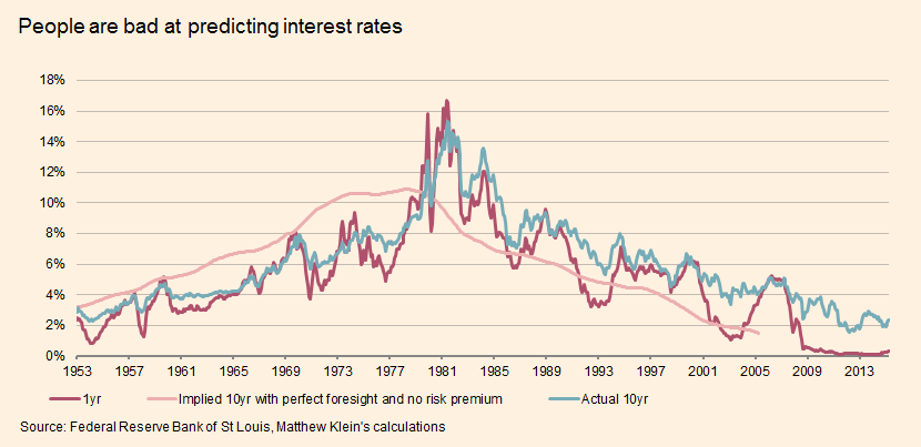
The following graph from the post struck me as very useful, especially as so much bond discussion tends to have short memories.

If the 10 year rate had followed the pink line,  you would not have made any more buying 10 year bonds than buying short term bonds. (The pink line is the forward-looking moving average of the one year rates.)

What the graph shows beautifully, then,  is this: Until 1981, long-term bonds were awful. You routinely lost money buying 10 year bonds relative to buying one year bonds. It goes on year in and year out and starts to look like a constant of nature.

From 1981 until today, the actual 10 year rate has been well above this ex-post breakeven rate. It's been a great 35 years for long-term bond investors. That too seems like a constant of nature now.

Of course, inflation going down was good for long term bonds. But we usually don't think there can be surprises in the same direction 35 years in a row.


You can also see the steady 35 year downward trend in 10 year rates. Good luck seeing the "massive" effects of quantitative easing or much of anything else here.

A lot of academic papers are devoted to this risk premium in bonds, including "Decomposing the yield curve" that I wrote with Monika Piazzesi.

It is now routine to decompose the spread between long and short term bonds into an expectations component and a risk premium, with changes in risk premium accounting for "conundrums." It is also routine not to present standard errors of this decomposition. The one thing I know for sure is that there is a lot of uncertainty on that decomposition. Any risk-premium estimate comes down to a bond-return forecasting regression. We know how much uncertainty there is in that exercise.

Sargent on Friedman

I ran across a little gem by Tom Sargent, "The Evolution of Monetary Policy Rules." Alas, it's gated in the JEDC so you'll need a university IP address to read it, and I haven't found a free copy. It's a transcript of a talk, so doesn't have Tom's usual prose polish, but insightful nonetheless.

Milton Friedman, like the rest of us, changed his mind over the course of a lifetime.

Coordinating monetary and fiscal policy:

...At different times, Friedman advocated two apparently polar opposite recommendations. In Friedman (1948), he proposed the following rule. He recommended to the fiscal authorities that they run a balanced budget over the business cycle. And he said what the monetary authorities should do, whatever the fiscal authority does, is to monetize 100% of government debt. That monetary rule implies that the entire government deficit is going to be financed with money creation. That is it.

It is interesting to contemplate what Friedman׳s monetary policy rule would imply if the fiscal authority chooses to deviate from Friedman׳s fiscal recommendation by running sustained deficits over the business cycle. Friedman׳s monetary rule then throws responsibility for inflation control immediately at the foot of the fiscal authority. Friedman׳s (1948) monetary rule tells the fiscal authority that if it wants stable money, then it better do the right things. If you want a stable price level, you had better recognize that you need a sound fiscal policy, period.  The division of responsibilities between monetary and fiscal authorities is clearly and unambiguously delineated. It is a completely clean set of rules. And this is what Friedman advocated until 1960.

Friedman (1960) advocated what looks to be exactly an opposite set of rules for coordinating monetary and fiscal policy. Friedman now advocated that the Federal Reserve, come hell or high water – it is not a Taylor Rule (for technical reasons) – should increase high-powered money, or something close to it, at k-percent a year, where k is the growth rate of the economy. The Fed is told to stick to the k-percent rule no matter what, recession or no recession. Under this rule, the arithmetic of the government budget constraint will force the fiscal authority to balance its budget in a present value sense.

What is beautiful about both sets of rules, the 1948 set and the 1960 set, is that they are both very clear descriptions of the lines between monetary and fiscal policy. But the rules ascribe quite different duties to the monetary [and fiscal! - JC] authority.

The line between money and credit

... In his 1960 A Program for Monetary Stability, and also earlier, Friedman embraced the Chicago tradition of 100% reserves for banks, namely, institutions that offer perfect substitutes for government currency. This amounts to setting an iron curtain line between money and credit. Here is the classic Chicago justification: If you want price level stability, you want to prevent shocks that originate in the borrowing and lending markets from impinging on the supply or demand for money. If you want to do that, just do it: 100% reserves basically puts anybody who issues anything that looks like money out of the business of intermediating. But then who intermediates? It would be firms that engage in the business of servicing lenders who are willing to chase higher returns than offered by money by taking term structure and investment risks. That is a socially desirable business, but according to the 100% reserves rule, it is not what banks or the monetary authority should do.

As someone given to qualifying his recommendations, on the very page that he recommends the 100% reserves rule, Friedman cites in a footnote an unpublished paper by Becker (1956) that convinced Friedman that 100% reserves may be exactly the opposite of what you should do. Instead, you should have free banking, but not like Michael Bordo (2014) described in this conference volume. Becker and Friedman really meant free banking. No charters. Free entry. Let anybody issue bank notes if that they want and let the market value them. That is very much like Adam Smith׳s recommendation in the “Wealth of Nations”. In the footnote, Friedman said Becker and Smith might be correct. Then in the text, Friedman proceeded to discuss how you might finance the interest at a market rate that he recommended be paid on those 100% reserves. He said that how you finance those interest payments is an important issue that will affect outcomes.

So even when he recommended one position, Friedman respectfully entertained a diametrically opposed one. Actually, near the end of his professional life, in one of the last papers he wrote with Anna Schwartz, Friedman virtually endorsed free banking, adding some nice words about Hayek (Friedman and Schwartz, 1986).

Is this waffling? No.

Again, the reason I mention Friedman׳s shifting positions is that superficially they seem to be diametrically opposed. They are united at a deeper level by their respect for government inter-temporal budget constraints and their clear division of responsibilities. They are very clear proposals. They’re not ambiguous. They are definite rules. You do not need a dynamic stochastic general equilibrium model to write them down or describe them. But technically, in the instructions to monetary authorities and regulators, they seem to be opposite.

Notice that Friedman does not recommend adopting “something in the middle” – that would confuse issues and only expand a mischievous role for exceptions and “judgment”.

What I take away from all of this is that if Milton Friedman thought that these are tough questions to decide, then they probably are. And they are not going to go away. And if Milton Friedman chose to spend a lot of time thinking about them, then they are probably very important problems to study and resolve.

The rest of the talk is good too, but I've surely exceeded the proper limit for lifting quotes.

Learning and New Keynesian Models.

John Barrdear at the Bank of England just posted an interesting paper, Towards a New Keynesian theory of the price level. Like Garcia Schmidt and Woodford, it changes the information structure of the standard model to avoid the standard model's problems.

Modifying the standard New-Keynesian model to replace firms' full information and sticky prices with flexible prices and dispersed information, and imposing mild and plausible restrictions on the monetary authority's decision rule, produces the striking results that (i) there exists a unique and globally stable steady-state rate of inflation, despite the possibility of a lower bound on nominal interest rates; and (ii) in the vicinity of steady-state, the price level is determinate (and not just the rate of inflation), despite the central bank targeting inflation. ... The model admits a determinate, stable solution with no role for sunspot shocks when the monetary authority responds by less than one-for-one to changes in expected inflation, including under an interest rate peg....

I haven't read this one yet either. I'm posting for anyone following these issues. Like Garcia Schmidt and Woodford, I also hope that others will read the papers and help to figure out if they really work as advertised.

Behavioral Public Choice

In a number of blog posts, (here ) I've complained about the lack of behavioral public choice theory, and highlighted some efforts in that direction.

Much behavioral economics documents that people do stupid things, and then jumps to the conclusion that parternalistic government can do things for us better. But wait, those government functionaries are also human, also behavioral, and placed in group and social settings that psychology as well as economics warns us are particularly prone to bad outcomes.

Marginal revolution highlights an interesting new paper that breaks in to this field, Behavioral public choice: The behavioral paradox of government policy by Ted Gayer and W. Kip Viscusi. A quote:

In this article we examine a wide range of behavioral failures, such as those linked to misperception of risks, unwarranted aversion to risk ambiguity, inordinate aversion to losses, and inconsistencies in the tradeoffs reflected in individual decisions. Although such shortcomings have been documented in the behavioral literature, they are also reflected in government policies, both because policymakers are also human and because public pressures incorporate these biases. The result is that government policies often institutionalize rather than overcome behavioral anomalies.

I haven't read it, but it seems interesting, and the field seems wide open. The defense of freedom never was that freedom is perfect, merely that government control is worse.

I am interested that behavioral economics seems so focused on mistakes of individual decision making, as nicely summarized in the quote. In fact the most obvious thing about humans is that we are social animals, not that we are poor individual decision-makers. I would think that behavioralists would be bringing social psychology more than individual decision making to economics. But maybe this just reveals how little I know about either.

Garcia Schmidt and Woodford on neo-Fisherian economcs

Mariana Garcia Schmidt and Mike Woodford are lighting up the internet with a presentation on neo-Fisherian economics -- the proposition that, when we are satiated in money as at the zero bound or with interest on reserves, raising interest rates raises inflation. Noah Smith, Marginal Revolution, Brad DeLong, and indirectly at Mark Thoma's econbrowser.

This is a particularly important voice, as it seemed to me that standard New-Keynesian models produce the new-Fisherian result. i = r + Epi is a steady state in all models. In old-Keynesian models, it was an unstable steady state, so an interest rate peg leads to explosive inflation or deflation. But in new-Keynesian models, an interest rate peg is the stable/indeterminate case. There are too many equilibria, but if you raise interest rates, inflation always ends up rising to meet the higher interest rate.

What I can glean from the slides is that Garcia Schmidt and Woodford agree: Yes, this is what happens in rational expectations or perfect foresight versions of the new-Keynesian model. But if you add learning mechanisms, it goes away.

My first reaction is relief -- if Woodford says it is a prediction of the standard perfect foresight / rational expectations version, that means I didn't screw up somewhere. And if one has to resort to learning and non-rational expectations to get rid of a result, the battle is half won.

But that's only preliminary relief. Schmidt and Woodford promise a paper soon, which will undoubtedly be well crafted and challenging.

For more on the issue, here is a a previous blog post. Section 3.1 ff of "Monetary policy with interest on reserves" has a full new Keynesian model with the Fisherian result. And a wry prediction: the Fed will raise rates to head off inflation, that will cause the inflation, then the Fed will congratulate itself on having headed off the inflation.  I also suspect that models with restricted liquidity (no interest on reserves) do give a temporary decline in inflation, but without that liquidity we now will get full Fisherian results. But that's just a conjecture so far.  My last foray into learning in new-Keynesian models, which didn't end well.

Why post now? Garcia Schmidt and Woodford clearly will have a thoughtful and sophisticated paper, on what I think is a deep and important point. I hope to encourage others to read and help to digest the paper.

China crash?

Meanwhile, on the other side of the world, China is doing everything in the textbook to ignite a "bubble."

I dislike that usually undefined term, which carries a lot of normative baggage. But there are a set of steps that governments often take unwittingly and are later criticized for. China's doing them on purpose. And these steps quite often precede large market declines.

Short sales ban: Financial Times: "opened a probe into market manipulation"  ... "The investigation is likely to focus on short selling."  The usual witch hunt, with Chinese characteristics. Owen Lamont has a splendid paper on what often follows short-sales bans. The weekend before TARP and Lehman, the US instituted a short-sales ban on bank stocks, just in case there was someone out there who did not know banks were in trouble and they should sell now. Europe instituted a CDS selling ban in the first PIGS crisis...

Lending to encourage highly leveraged speculation: Wall Street Journal: "Under the planned move, China’s central bank will indirectly help investors borrow to buy shares in a market that had already seen a rapid buildup in debt from so-called margin financing." Procyclical credit supply is named by just about every account of a "bubble" followed by a crash.

Prices depend on supply and demand. As well as increasing demand, limit supply: "A halt to new stock listings."

And more. Quartz offers "A complete list of the Chinese government’s stock-market stimulus (that we know about)" including  "People’s Bank of China will “provide liquidity assistance” to China Securities Finance Corp., a company owned by the stock regulator. The company will use the money to lend to brokerages, which could then make loans to investors to buy stocks."

This scenario often ends badly.

The only thing I can think of that can actually stop a crash is for the central bank to directly print money to buy stocks. And not just a little bit. A pre-announced and limited quantity won't work. The US QE took billions to alter bond prices a few basis points at most. One has to commit to a price floor and a "do what it takes" amount of money, no matter how large or inflationary. I don't know of it ever being tried. It will be interesting to see if China goes that far. They could hide the fact with extensive bailouts of people "borrowing" to buy stocks, or otherwise cover losses or promise to cover losses.

Of course, the right strategy is to leave it alone. The whole point of stocks is that they go down on occasion, without runs, without defaults, and without financial distress. Unless the people and institutions holding them are highly leveraged. Didn't we just learn this lesson?

Noah Smith Writing Lesson

Source Noah Smith

Noah Smith has a good review of the writing in Deirdre McCloskey's review of Thomas Piketty's book.

A lesson for students learning to write papers: Don't needlessly annoy readers before you get to your point. If a reader disagrees, finds something wrong, or insufficiently documented, of if you offend a reader, he or she will leave without getting to the main point.  Once a reader finds one thing he or she thinks is wrong, he or she will distrust the rest of the argument. Grand methodological statements and criticisms of swaths of literature are especially dangerous.

Noah's post is a great example. As you can see, Noah never got to the main point of McCloskey's review, and happily admits it.

And Noah's criticisims are spot on.  The first four pages of McCkoskey's review are full of grand, outrageous, and arguably false statements, having nothing to do with Piketty, inequality, or anything else that follows.  McCloskey, author of a splendid essay on writing in economics, should really have known better.  My review said as much too. Interestingly, I quoted quite a few of the same points Noah found.  (I put that at the bottom of a "too-long post on a far-too-long review of a enormously-too-long book" because  my main point was not about writing and for once I followed my own advice and put the secondary point at the bottom.)

So, dear students, learn the lesson: write the minimum up front needed to make your main point later. If you think everyone runs too many regressions, or you don't like non-cooperative game theory, and unless this point is absolutely necessary to your criticism of Piketty, save it for another day. Only offend people you really really need to offend. Otherwise, you risk having a potential reader like Noah give up in disgust before he gets to your point. Noah, hold your nose and plow on, it gets better.

Unit roots in English and Pictures

After my unit roots redux post, a few people have asked for a nontechnical explanation of what this is all about.

Suppose there is an unexpected movement in any of the data we look at -- inflation, unemployment, GDP, prices, etc.  Now, how does this "shock" affect our best estimate of where this variable will be in the future? The graph shows three possibilities.


First, green or "stationary."  There may be some short lived dynamics, the little hump shape I drew here. Then, given enough time, the variable will return to where we thought it was going all along. For unemployment, suppose your best guess of unemployment in 2050 was 5%. Then you see an upward unexpected 1% spike in today's unemployment. Ouch, that means that we're going back to a recession. But perhaps this news does not change your view of 2050 unemployment at all.

Second, blue or "pure random walk." That's more plausible (though no longer thought to be true) of stock prices. If the price goes up unexpectedly, your expectation of where the (log) price will be in the future goes up one-for-one, for all time.

Third, black, "unit root." This option recognizes the possibility that a shock may give rise to transitory dynamics, and may come back towards, but not all the way towards your previous estimate. As you can see the "unit root" is the same as a combination of a stationary component and a bit of a random walk. Perhaps seeing unemployment rise 1%, you think most of it will work itself out, but that even in the long run labor markets will be sticky and we'll never quite get back.

The "unit root" is most plausible and verified in the data for log GDP. Recessions and expansions have a lot of transitory component that will come back. But there are permanent movements too. Unemployment, being a ratio, strikes me as one that eventually must come back. But it can take a longer time than we usually think, which is interesting.

This is very simplified. A few of the issues:

For GDP the question is whether it will come back to a linear trend extrapolated from past data, not back to a level as I have shown.

Most of the issue is how standard statistical procedures work in these circumstances.

As you can see from the graph, the pure question whether the series will come back in an infinite time period is not really knowable. It could be that the series will come back eventually, but take a very long time. It could be stationary plus a second very slow moving stationary component. This is a statistical problem but not really an economic problem. The appearance of unit roots are economically interesting as they show a lot of "low frequency" movement, series that are coming back slowly -- even if they do come back eventually. The economics of "slumps" and (we hope, someday) "booms" is hot on the agenda, and this is one indication of the fact.

This is all much more interesting if you look at multiple series together. For the canonical example, if you just look at stock prices, they are very very close to a random walk. A price rise or decline are permanent. However, if you see stock prices rise relative to dividends, that's almost entirely stationary. GDP and consumption have a similar relationship. As in the latest recession, if GDP declines with a big consumption decline, that looks pretty darn permanent. GDP declining and people still consuming is much more likely to go away.

I hope this helps.

Consumption-based model and value premium

The consumption based model is not as bad as you think. (This is a problem set for my online PhD class, and I thought the result would be interesting to blog readers.)

I use 4th quarter to 4th quarter nondurable + services consumption, and corresponding annual returns on 10 portfolios sorted on book to market and the three Fama-French factors. (Ken French's website)

The graph is average excess returns plotted against the covariance of excess returns with consumption growth. (The graph is a distillation of Jagannathan and Wang's paper, who get any credit for this observation.  The lines are OLS cross-sectional regressions with and without a free intercept.)


By comparison, the CAPM is the usual disaster. If we plot average returns against the covariance of returns with the market (rmrf) or against market betas, there is very little pattern. In particular, the hml portfolio, which by itself captures almost all the pricing information in the ten b/m portfolios (that's the point of the Fama-French model) has a 5% average return and a slightly negative market beta. The fact that the hml portfolio is right on the line in the previous graph is the main point of that graph.

There is an essentially correct story in the consumption-based model: value stocks and small stocks have higher average returns. And they have correspondingly higher covariance with consumption growth. Value and small stocks tend to do poorly in years of bad consumption growth, though they have little systematic correlation with the market.

Is this perfect? No. The model is \(E(R^e) = cov(R^e, \Delta c)) \times \gamma\) where \(R^e\) = excess return, \(\Delta c\) is consumption growth and \( \gamma\) is the risk aversion coefficient. The mean returns are so large -- and the volatility of consumption growth so small -- that the slope coefficient = risk aversion coefficient is 80, a bit hard for most people to swallow.

Also, this is the linearized model. The true nonlinear model is \(E(R^e) = -cov(R^e_{t+1}, (c_{t+1}/c_t)^{-\gamma})\), and raising things to the 80th power is a lot different than multiplying by 80. On the other hand, perhaps this is the key to good performance. If you think the underlying correct model works in continuous time,  which is linear, \( E_t(dR^e) = -E_t(dR^e, dc)  \gamma \), then perhaps the linearized model is a better approximation to annual time-averaged data than is the discrete-time model that pretends all consumption happens in one big lump every December 31. Furthermore, if you raise consumption growth to the 80th power, all the covariance of returns with marginal utility comes in one or two big spikes. The model becomes a model of rare disasters in marginal utility, not one of repeated events. Perhaps, but life would be so much easier if markets were about repeated risks not once per century disaster covariances.

The larger point: Very few researchers have really given the consumption model a good go to see just how full the glass might be. Hansen and Singleton famously rejected the model, but they used monthly seasonally adjusted consumption data, a bunch of low-power instruments, and no treatment of time aggregation (consumption is sum for the month, returns are 30th to 30th), or the durability of most "nondurable" goods. (Shirts are "nondurable." I get all mine at Christmas, hence 4th quarter to 4th quarter works pretty well for me!) Their point was mostly an illustrative example of GMM methodology not a serious Fama-French style empirical investigation of just how far a model can go. (The Fama-French model is also rejected!) It took 25 years before Jagannathan and Wang produced this simple graph. Can we do even better?

Sure, the consumption-based model won't work at a 5 minute interval. But is there some essence of truth in it, that stocks which fall more in business cycles, as measured by consumption, must pay a higher rate of return.  Just how far does that truth go? I think one could do far better by thinking hard about time aggregation,  data construction, durability, seasonal adjustment, and the appropriate frequency to evaluate such a model. And by trying to see just how far the model can go, rather than statistically rejecting its perfection.

In the end  "why are people afraid of value stocks and leave attractive returns on the table?" must come down to 1) they're morons, they haven't figured it out 2) the value premium isn't really there or 3) value stocks do badly in bad times, so make a portfolio riskier. That consumption is also low in these bad times seems pretty natural.

Update

From "Cross-Sectional Consumption-Based Asset Pricing: A Reappraisal" by Tom Engsted and Stig Vinther Møller at University of Aarhus. Thanks to Stig for the link. BOP and EOP are beginning of period and end of period consumption. In a discrete time model, do you treat the sum of consumption over the year as happening at the beginning of the year, or the end of the year? Treating it at the beginning produces the dramatic graph on the left.

This is a small instance of the many explorations one can do to see if there is some power to the consumption-based model, rather than just take it literally and reject it.

A bigger point. Means are pretty insensitive to timing. But covariances and correlations of white noise series are exquisitely sensitive to timing, measurement error, and so forth. \(cov(a_t,b_t)\) may be large, and \( cov(a_{t-1} b_t)=0\). Another approach is to create time averaged returns. I did this a long time ago here. Average january-january, feburary-february, march-march, etc. returns and compare them to the growth of annual macro data. The right thing to do is to explicitly model time aggregation -- the fact that consumption is reported as an annual average -- along with seasonal adjustment.

Macro Handbook 2

Last week I attended the first half of the conference on the Handbook of Macroeconomics Volume 2, organized by John Taylor and Harald Uhlig, held at Hoover. The conference program and most of the papers are here.  The second half will be in Chicago April 23-25, program here

Overall, this Handbook is shaping up as a very useful resource.  Really good summary and review papers are a natural way in to long literatures. Bad summary and review papers are long and boring. The conference produced the first kind. Most of the papers are rough first drafts, so make a note to come back when they're finished. A few highlights (with apologies to authors I've left out; I can't review them all here.)


Chad Jones' "The Facts of Economic Growth" is a tremendous introduction to a complex field, nicely mixing facts and ideas. If you last left growth theory with a view that ratios are stable and we just climb up with TFP, this paper will change that view. Equipment is getting cheaper. Factor shares are moving. Human capital is trending up, along with its price. R&D spending and employment share trend up. Misallocation has first-order negative effects on productivity, a finding from growth theory that macro should pay more attention to. Agriculture is declining, health care expanding. Fertility is declining. Inequality, .. yes, that too. Sometimes countries converge, sometimes they diverge.

"... once countries get on the “growth escalator,” good things tend to happen and they grow rapidly to move closer to the frontier. Where they end up depends, as we will discuss, on the extent to which their institutions improve."

Jesús Fernández-Villaverde, Juan Rubio-Ramirez and Frank Schorfheide's  "Solution and Estimation Methods for DSGE Models" is encyclopedic, approaching a book in itself. The technique of solving models, curiously banished from papers these days, is a dark art. There are lots of techniques. Which do you use when?  think this will be a very useful "cookbook" for modelers, which is just the sort of thing handbooks are good for. We had a lively discussion on which techniques are best for which kinds of models. How many shocks, how many state variables, how important are nonlinearities all matter. I made the usual complaints about identification, and that perhaps models we know are false (one shock, many series) might not be right for formal black box estimation methods. Intuitive connection to robust facts in the data may be more important than statistical efficiency when the model is a quantitative parable.

Monica Piazzesi Martin Schneider's "Housing and Macroeconomics" -- no paper yet, alas, but look for it --  is a very nice introduction to the kind of explicit modeling interacted with data that they've been doing.

Valerie Ramey's  Macroeconomic Shocks and Their Propagation took up the current state of vector autoregressions, shock identification and so forth. A great integration of a long literature. Where are we?  Both Valeire and Arvind Krishnamurthy discussing showed lots of graphs with varying signs of the effects of monetary policy. Despite sixty years (since Milton Friedman regressed output on money, with high points from Tobin and Solow early 1960s; St. Louis Fed late 1960s;  Sims and Granger late 1970s;  Christiano-Eichenbaum-Evans 1999; Romer and Romer more recently), we're still at it.  Most of the discussion pointed out how much uncertainty there still is. I opined that most of the "uncertainty" was about how much you have to torture estimates to avoid the conclusion that interest rate rises raise output and inflation.

Gary Hansen and Lee Ohanian cover "Neoclassical Theories" by example, integrating three recent models they have worked on, covering how "neoclassical" theories can account for the Great Depression, the WWII boom, and the surprisingly large postwar fluctuations at frequencies lower than standard business cycles. My discussion complained about the habit of different models for different facts, and exogenous TFP shocks. I suggests that it's time to view business cycle TFP movements as more than just scientific innovation identified by residual, but rather to include and independently measure all the "wedges" that policy is inducing between invention and adoption. Among other points.

Jim Stock and Mark Watson, "Factor Models for Macroeconomics" (No paper, alas, but look for it) is shaping up to be one of those very useful "how to" papers that handbooks can provide. Lots of insight in how to use the Stock-Watson methodology in many contexts, all in one place, and (to judge by Mark's presentation) ultra-clear and accessible.

Bob Hall closed strong with "Macroeconomics of Persistent Slumps," the latest in Bob's thinking on this subject (other highlights are his AEA Presidential Speech and Macro Annual paper.) An interesting sidelight, Bob also innovated a new solution methodology. Write the shocks as multinomials, then just solve first order conditions on the following tree. It's amazingly fast. And not in the Fernández-Villaverde,  Rubio-Ramirez, Schorfheide cookbook.

Again, the other papers were great too. And the second round promises to equal if not better the first.

The sources of stock market fluctuations

How much do dividend-growth vs. discount-rate shocks account for stock price variations?

An under-appreciated point occurred to me while preparing for my Coursera class and to comment on Daniel Greewald, Martin Lettau and Sydney Ludvigsson's nice paper "Origin of Stock Market Fluctuations" at the last NBER EFG meeting

The answer is, it depends the horizon and the measure. 100% of the variance of price dividend ratios corresponds to expected return (discount rate) shocks, and none to dividend growth (cash flow) shocks.  50% of the variance of one-year returns corresponds to cashflow shocks. And 100% of long-run price variation corresponds to from cashflow shocks, not expected return shocks. These facts all coexist

I think there is some confusion on the point. If nothing else, this makes for a good problem set question.

The last point is easiest to see just with a plot. Prices and dividends are cointegrated. Prices correspond to dividends and expected returns. Dividends have a unit root, but expected returns are stationary. Over the long run prices will not deviate far from dividends. So 100% of long-enough run price variation must come from dividend variation, not expected returns.

Ok, a little more carefully, with equations.

A quick review: 

The most basic VAR for asset returns is \[ \Delta d_{t+1} = b_d \times dp_{t}+\varepsilon_{t+1}^{d} \] \[ dp_{t+1} = \phi \times dp_{t} +\varepsilon_{t+1}^{dp} \] Using only dividend yields dp, dividend growth is basically unforecastable \( b_d \approx 0\) and \( \phi\approx0.94 \) and the shocks are conveniently uncorrelated. The behavior of returns follows from the identity, that you need more dividends or a higher price to get a return,  \[ r_{t+1}\approx-\rho dp_{t+1}+dp_{t}+\Delta d_{t+1}% \] (This is the Campbell-Shiller return approximation, with \(\rho \approx 0.96\).) Thus, the implied regression of returns on dividend yields, \[ r_{t+1} = b_r \times dp_{t}+\varepsilon_{t+1}^{r} \] has \(b_r = (1-\rho\phi)+0 = 1-0.96\times0.94 = 0.1\) and a shock negatively correlated with dividend yield shocks and positively correlated with dividend growth shocks.

The impulse response function for this VAR naturally suggests "cashflow" (dividend) and "expected return" shocks, (d/p). (Sorry for recycling old points, but not everyone may know this.)

Three propositions:

• The variance of p/d is 100% risk premiums, 0% cashflow shocks

Iterate forward the return identity, to get \[ dp_{t} =\sum_{t=1}^{\infty}\rho^{j-1}r_{t+j}-\sum_{t=1}^{\infty}\rho ^{j-1}\Delta d_{t+j} \] multiply by \(dp_t\) and take expectations (all variables are demeaned) \[\sigma^{2}\left( \log\frac{P_{t}}{D_{t}}\right) =\sigma^{2}\left( dp_{t}\right) =\sum_{t=1}^{\infty}\rho^{j-1}cov(dp_{t},r_{t+j})-\sum _{t=1}^{\infty}\rho^{j-1}cov(dp_{t},\Delta d_{t+j}), \] But \(b_d \approx 0 \), so the dividend growth terms are all zero, and 100% of the variance of price-dividend ratios corresponds to time-varying expected returns. (I know this will bore people familiar with it and befuddle those who are not. "Discount rates" has a bit more leisurely review and citations)

 But

•  The variance of returns is 50% due to risk premiums, 50% due to cashflows. 

\[ r_{t+1}=-\rho dp_{t+1}+dp_{t}+\Delta d_{t+1}% \] \[ \varepsilon_{t+1}^{r} =-\rho\varepsilon_{t+1}^{dp}+\varepsilon_{t+1}^{d} \] \[ \sigma^{2}\left( \varepsilon_{t+1}^{r}\right) =\rho^{2}\sigma^{2}\left( \varepsilon_{t+1}^{dp}\right) +\sigma^{2}\left( \varepsilon_{t+1}^{d}\right) \] The variance of the two shocks comes out very close to a 50/50 decomposition at an annual horizon. It's a lot more expected return at a daily horizon, and less at longer horizons. Here I use the fact that dividend growth and dividend yield shocks are basically uncorrelated.

Why are returns and p/d so different?  Current cash flow shocks affect returns. But a shock to dividends, when prices rise at the same time, does not affect the dividend price ratio. (This is the essence of the Campbell-Ammer return decomposition.)

The third proposition is less familiar:

• The long-run variance of stock market values (and returns) is 100% due to cash flow shocks and none to expected return or discount rate shocks.

Here's why: \[ \Delta p_{t+1} =-dp_{t+1}+dp_{t}+\Delta d_{t+1} \] \[ p_{t+k}-p_{t} =-dp_{t+k}+dp_{t}+\sum_{j=1}^{k}\Delta d_{t+j} \] so as k gets big, \[ {var} (p_{t+k}-p_{t}) \rightarrow 2 {var}(dp_t) + k {var}(\Delta d_{t}) \] The first term approaches a constant, but the second term keeps growing. As above the central fact is that P and D are cointegrated while expected returns are stationary.

This is related to a point made by Fama and French in their Equity Premium paper. Long run average returns are driven by long run dividend growth  plus the average value of the dividend yield. The difference in valuation -- higher prices for given set of dividends -- can affect returns in a sample, as higher prices for a given set of dividends boost returns. But that mechanism can't last. (Avdis and Wachter have a nice recent paper formalizing this point.)  It's related to a similar point made often by Bob Shiller: Long run investors should buy stocks for the dividends.

A little more generality as this is the new bit.

\[ p_{t+k}-p_t = dp_{t+k}-dp_t + \sum_{j=1}^{k}\Delta d _{t+j} \] \[ p_{t+k}-p_t = (\phi^{k}-1)dp_t + \sum_{j=1}^{k}\phi^{k-j} \varepsilon^{dp}_{t+j} +  \sum_{j=1}^{k} \varepsilon^d _{t+j} \] \[ var(p_{t+k}-p_t) = \frac{(1-\phi^{k})^2}{1-\phi^2} \sigma^2(\varepsilon^{dp}) + \frac{(1-\phi^{2k})}{1-\phi^2}  \sigma^2(\varepsilon^{dp}) +  k\sigma^2(\varepsilon^d) \] \[var(p_{t+k}-p_t) = 2\frac{(1-\phi^{k})}{1-\phi^2} var(\varepsilon^{dp}_{t+1})  + k var(\varepsilon^d_{t+j})\] So you can see the last bit takes over. It doesn't take over as fast as you might think. Here's a graph using sample values,

At a one year horizon, it's just about 50/50. The dividend shocks eventually take over, at rate 1/k. But at 50 years, it's still about 80/20.

Exercise for the interested reader/finance professor looking for problem set questions: Do the same thing for long horizon returns, \( r_{t+1}+r_{t+2}+...+r_{t+k} \) using \(r_{t+1} = -\rho dp_{t+1} + dp_t + \Delta d_ {t+1} \) It's not so pretty, but you can get a closed form expression here too, and again dividend shocks take over in the long run.

Be forewarned, the long run return has all sorts of pathological properties. But nobody holds assets forever, without eating some of the dividends.

Disclaimer: Notice I have tried to say "associated with" or "correspond to" and not "caused by" here! This is just about facts. The facts have just as easy a "behavioral" interpretation about fads and bubbles in prices as they do a "rationalist" interpretation. Exercise 2: Write the "behavioralist" and then "rationalist" introduction / interpretation of these facts. Hint: they reverse cause and effect about prices and expected returns, and whether people in the market have rational expectations about expected returns.

A New Structure for U. S. Federal Debt

A new paper by that title, here.

I propose a new structure for U. S. Federal debt. All debt should be perpetual, paying coupons forever with no principal payment. The debt should be composed of the following:

1. Fixed-value, floating-rate debt: Short-term debt has a fixed value of $1.00, and pays a floating rate. It is electronically transferable, and sold in arbitrary denominations. Such debt looks to an investor like a money-market fund, or reserves at the Fed. 
2. Nominal perpetuities: This debt pays a coupon of $1 per bond, forever. 
3. Indexed perpetuities: This debt pays a coupon of $1 times the current consumer price index (CPI).
4. Tax free: Debt should be sold in a version that is free of all income, estate, capital gains, and other taxes. Ideally, all debt should be tax free. 
5. Variable coupon: Some if not all long-term debt should allow the government to vary the coupon rate without triggering legal default. 
6. Swaps: The Treasury should manage the maturity structure of the debt, and the interest rate and inflation exposure of the Federal budget, by transacting in simple swaps among these securities.

Of these, I think the first is the most important. Think of it as Treasury Electronic Money, or reserves for all. Why?

Economists have long dreamed of interest-paying money. It fulfills Milton Friedman’s (1969) optimal quantity of money without deflation. Paper money is free to produce, so the economy should be satiated in liquidity...

Our economy invented inside interest-paying electronic money in the form of money market funds, overnight repurchase agreements, and short-term commercial paper, and found it useful. But that money failed, suffering a run in the 2008 financial crisis. Treasury-provided interest-paying electronic money is immune from conventional runs. Money market funds 100% backed by fixed-value Treasury debt cannot suffer a run...

By analogy, in the 19th century, the Treasury provided coins. Banks issued notes. Notes were convenient, being a lot lighter than coins. But there were repeated runs and crises involving bank notes. The U.S. government issued paper money, which might inflate, but cannot suffer conventional default or a run. That money eventually drove out private banknotes, and that source of financial crises was permanently ended. (Crises involving demand deposits did not end, but here the U.S. tried a different policy response, deposit insurance and risk regulation. It has not worked as well.)

In the 21st century, the Treasury has exactly the same natural monopoly in providing default-free and run-free electronically-transferable interest-paying money to private parties. It should do so.

If the Treasury offers what are essentially interest-paying reserves, then we don't have to argue about the size of the Fed's balance sheet, ON RRP, etc.

Nominal perpetuities are a nice way to condense the hundreds of outstanding issues into one, which should increase their liquidity a good deal.

Indexed perpetuities are a cleaner way to implement today's tips.

The tax free analysis is maybe the most interesting. I put together a little tax clientele model with some interesting results. No, issuing tax free debt is not a present to rich people. By attracting the high tax clientele back to Treasury debt, we should see lower net (after tax) interest costs to the Treasury.

I have a nice implementation of Treasury swaps too, that might open them up a lot.

Comments welcome. It's a bit long because it responds to a previous round of comments, so if you're bubbling over with what's wrong with the proposals, do check that I haven't already answered your comment.

Jumps and diffusions

I learned an interesting continuous time trick recently. The context is a note, "The fragile benefits of endowment destruction" that I wrote with John Campbell, about how to extend our habit model to jumps in consumption. The point here is more interesting than that particular context.

Suppose one time series \(x\), which follows a diffusion, drives another \(y\). In the simplest example, \[dx_t = \sigma dz_t \] \[ dy_t = y_t dx_t. \] In our example, the second equation describes how habits \(y\) respond to consumption \(x\). The same kind of structure might describe how invested wealth \(y\) responds to asset prices \(x\), or how option prices \(y\) respond to stock prices \(x\).

Now, suppose we want to extend the model to handle jumps in \(x\), \[dx_t = \sigma dz_t + dJ_t.\] What do we do about the second equation? \(y_t\) now can jump too. On the right hand side of the second equation, should we use the left limit, the right limit, or something in between?

The usual answer is to use the left limit. We generalize the model to jumps this way: \[dx_t = \sigma dz_t+ dJ_t \] \[ dy_t = y_{t_-} dx_t = y_{t_-} \sigma dz_t + y_{t_-}dJ_t \] where \(y_{t_{-}}\) denotes the left limit.

That approach has some weird properties however. Suppose \(y_{t_-}=1\), and \(dJ_t=1\). Then \(y_t\) jumps to \(y_t=2\). But suppose there are two jumps of size 1/2, one at time \(t\) and one at time \(t+\varepsilon\). Now \(y\) jumps up to 1.5 after the first jump, and then jumps another \(1.5 \times 0.5 = 0.75\), ending up at \(y_{t+\varepsilon} =2.25\). Two half jumps have a different response than one full jump.

Suppose instead we extend the original model to jumps by taking the jump limit of a continuous process. Imagine that we observe realizations of \(\{dz_t\}\) that get closer and closer to a jump in \(dx_t\), and let's find what happens to \(y_t\). The general solution to the first set of equations is \[ y_{t+\Delta} = y_t e^{(x_{t+\Delta}-x_t - \frac{1}{2}\sigma^2\Delta)}\] so, in the limit \(\Delta \rightarrow 0\) that \(x_t\) takes a jump of size \(dJ_t\), the jump-limit of a continuous movement is \[ dy_{t} \equiv y_t -y_{t_-} = y_{t_-}(e^{dx_{t}}-1) = y_{t_-}\sigma dz_t + y_{t_-}e^{dJ_t}\] rather than \[ dy_t = y_{t_-} dx_t = y_{t_-} \sigma dz_t + y_{t_-}dJ_t \] So, the left-limit method produced a response to a jump that was different from the response to a continuous process arbitrarily close to a jump. For example, the left-limit approach can produce a negative \(y_t\), but this method, like the diffusion process, cannot fall below zero. This method also produces a response to two half jumps that is the same as the response to a full jump.

As you can see, the difference is whether the state variable \(y_t\) gets to change during the jump. In the left-limit approach, the same \(y_{t_-}\) gets applied to the whole jump. In the continuous-limit version, \(y_t\) implicitly gets to move while the jump in \(x_t\) is moving.

A nonlinear function of a jump is a little novel, but there's nothing wrong with it, and it exists in the continuous time literature. We don't see it that often, because when you're only studying one series it's easier to just change the distribution of the jump process instead. This question occurs when you can see both series x and y and you want to model the relationship between them.

Which is right?

Which extension to jumps is correct? Both are mathematically correct. There is nothing wrong with writing down a model in which the response to a jump is different from the response to continuous movements arbitrarily close to jumps. The answer depends on the economic situation.

For example, consider models with bankruptcy constraints. Agents who can continuously adjust their investments may always avoid bankruptcy in a diffusion setting. If we extend such a model to jumps with the continuous limit approach, implicitly preserving the investor's ability to trade as fast as asset prices change even in the jump limit, we will preserve bankruptcy avoidance in face of a jump in prices. However, if we model portfolio adjustment to jumps with the left-limit generalization, agents may be forced in to bankruptcy for price jumps.

Sometimes, one introduces jumps precisely to model a situation in which prices can move faster than agents can adjust their portfolios, so agents may be forced to bankruptcy. Then the left-limit generalization is correct. But if one wants to extend a model to jumps for other reasons, while avoiding bankruptcy, negative consumption, negative marginal utility (consumption below zero or below habits), violations of budget constraints, feasibility conditions, borrowing constraints, and so forth, then one should choose a generalization in which the jump gives the same result as the continuous limit.

Similarly, when extending option pricing models to jumps, one may want to model the jump in such a way that investors cannot adjust portfolios fast enough. Then the left-limit extension is appropriate, and investors must hold the jump risk. But one may wish to accommodate jumps in asset prices to better fit asset price dynamics while maintaining investor's ability to dynamically hedge. Then the nonlinear extension is appropriate, maintaining the equivalence between jumps and the limiting diffusion.

A little more general treatment

A little more generally, suppose \[ dx_t = g dt + \sigma dz_t \] \[dy_t = \mu(y_t) dt + \lambda(y_t)dx_t.\] We want to add \(dJ_t\) to the first equation. The left-limit approach is \[dy_t = \mu(y_{t_-}) dt + \lambda(y_{t_-})dx_t \] If there is a jump \(dJ_t\), \(y\) moves by an amount \[\frac{1}{\lambda(y_{t_-})}dy_t \equiv \frac{1}{\lambda(y_{t_-})}(y_t - y_{t_-}) = dx_t .\] The limit of a continuous movement solves the differential equation \[\int_{y_{t_-}}^{y_t} \frac{1}{\lambda(\xi)}d\xi = dx_t\] Again, you see the crucial difference, whether the state variable gets to move "during" the jump. We can write this as a differential, by writing the solution to this last differential equation as \[y_t-y_{t_-}=f(x_t-x_{t_-};y_{t_-})\] and then \[dy_t = \mu(y_{t_-}) dt + f(dx_t;y_{t_-})=\mu(y_{t_-}) dt + \lambda(y_{t_-})\sigma dz_t+f(dJ_t;y_{t_-})\]

So, you don't have to extend the model to jumps with the left-limit approach, and you don't have to swallow the idea that a jump has a different response than an arbitrarily close continuous-sample-path movement. The last equation shows you how to modify the model to include jumps in a way that preserves the property that the jump has the same effect as its continuous limit.

The point

Why a blog post on this? I asked a few continuous-time gurus, and none of them had seen this issue before. If someone knows where this has all been worked out with proper is dotted and ts crossed, I would like to know and cite it properly. (I would think the literature on option pricing with jumps had done it, but I couldn't find a reference.) Or perhaps it hasn't been done and someone wants to do it. I'm not good enough at the technical aspects of continuous time to write this with the right precision and generality.

And it's a cool trick that may be useful to someone outside of the narrow context that we had for it.

Update: 

Perhaps the right application is stock prices and option prices. When stock prices jump, someone must have studied the case that option prices move by the same amount the Black-Scholes formula gives for the same size stock price movement. Does anyone have a citation to that case?

Borio, Erdem, Filardo and Hofmann on the Costs of Deflation

Claudio Borio, Magdalena Erdem, Andrew Filardo and Boris Hofmann have a nice paper, "The costs of deflations: a historical perspective"

Deflation remains the looming zombie apocalypse of international monetary commentary.  Before we argue too much about cause and effect, it's nice to get the correlations straight. And the correlation between deflation and poor growth is much weaker than most people think:

The authors:

...Price deflations have coincided with both positive and clear negative growth rates (Graph 2). And a comparison of all inflation and deflation years suggests that, on balance, inflation years have seen only somewhat higher growth (Table 2). The difference in average growth rates is highest and statistically significant only during the interwar years, particularly in the period 1929-38 that includes the Great Depression (some 4 percentage points), and much smaller at other times.... Indeed, in the postwar era, in which transitory deflations dominate, the growth rate has actually been higher during deflation years, at 3.2% versus 2.7%.

Really, the concern at the moment is not a sharp large deflation, such as occurred in the 1930s and is felt by many to epitomize the demand or debt deflation story. Rather, the concern is over a moderate but persistent deflation, such as Japan has experienced. (One in which each individual is likely to never experience a wage decline, more here.)

To summarize the historical record surrounding persistent deflations, the authors organize the data around the peak in CPI before a deflation episode, and show average CPI and GDP around that peak:

The authors:

 While mean growth rates are mostly lower in the five years post-peak, the difference is large, 3.6 percentage points, and clearly statistically significant (i.e.cannot be attributed purely to chance) only in the interwar years, when the Great Depression took place...The difference during the classical gold standard period is 0.6 percentage points but it is not statistically significant. In fact, in the postwar era, average growth was even 0.3 percentage points higher in the five years after a price peak, although the difference is not statistically significant. Moreover, only in the interwar years did output actually fall post-peak.

In a multiple regression sense, does variation in output correlate better with falls in the overall price level, or with falls in house prices or equity prices that accompany deflation?

The graph presents regression coefficients. Read it as the partial correlation, if (blue) property prices go down but consumer and equity prices do not, how much output gain or loss does that event signal?House price or stock price "deflation," not overall price deflation matters. Of course, stock prices and property prices are strong symptoms of economic trouble, so don't be quick to read causality into correlation and ask the Fed to punch up stock and house prices.

The introduction offers a corrective that every financial journalist should take with morning cappuccino. Any price change can come from supply or demand, and is as likely a symptom as a cause:

Concerns about deflation - falling prices of goods and services - have loomed large in recent policy discussions. The debate is shaped by the deep-seated view that deflation, regardless of context, is an economic pathology that stands in the way of any sustainable and strong expansion. 

The almost reflexive association of deflation with economic weakness is easily explained. It is rooted in the view that deflation signals an aggregate demand shortfall, which simultaneously pushes down prices, incomes and output. But deflation may also result from increased supply. Examples include improvements in productivity, greater competition in the goods market, or cheaper and more abundant inputs, such as labour or intermediate goods like oil. Supply-driven deflations depress prices while raising incomes and output.

Conversely, note the simultaneous worry in the US about "wage inflation" and that wages have stagnated. Wage inflation with stable prices is a good thing!

A minor quibble: Asset price "inflation" and "deflation."

Moreover, while the impact of goods and services price deflations is ambiguous a priori, that of asset price deflations is not. As is widely recognised, asset price deflations erode wealth and collateral values and so undercut demand and output.

First, "asset price inflation" sounds sexy, but our first duty as economists should be to help readers understand that relative price changes are not inflation. All relative price changes, including asset prices, are relative price changes, not inflations and deflations. Health cost "inflation," wine "inflation" and chewing gum "inflation" are not inflation. Don't encourage misuse of the word, misunderstanding of relative prices vs. price level, and consequent policy mistakes like using anti-inflation tools to manipulate relative prices.

Second, asset price "deflations" are in large part a transfer of wealth, not a loss of wealth. House prices go down. The houses are still there. This is a qualitatively different fact than if houses wash in to the ocean. If you are young, live in an apartment, and have a job, a house price decline is a great thing. If you plan to buy the same size house as you want to sell, a house price decline is a wash. If you are young, a bond price decline is a great thing. You get the same future payments at a lower price. To some extent the same is true of many stock price movements.

Arezki, Ramey, and Sheng on news shocks

I attended the NBER EFG (economic fluctuations and growth) meeting a few weeks ago, and saw a very nice paper by Rabah Arezki, Valerie Ramey, and Liugang Sheng, "News Shocks in Open Economies: Evidence from Giant Oil Discoveries" (There were a lot of nice papers, but this one is more bloggable.)

They look at what happens to economies that discover they have a lot of oil.

An oil discovery is a well identified "news shock."

Standard productivity shocks are a bit nebulous, and alter two things at once: they give greater productivity and hence incentive to work today and also news about more income in the future.

An oil discovery is well publicized. It incentivizes a small investment in oil drilling, but mostly is pure news of an income flow in the future. It does not affect overall labor productivity or other changes to preferences or technology.

Rabah,Valerie, and Liugang then construct a straightforward macro model of such an event.

Utility comes from consumption and work. The production function has an oil sector and non-oil sector. There are adjustment costs to investment and to reallocation of capital between oil and non-oil sectors. The consumption good is tradeable, and the economy sells oil internationally to get it as well as to produce it.

They compute impulse-response functions to big oil discoveries, and compare the model dynamics to the response functions. It's a nice fit and an intuitive story. After the shock hits, during the period of investment, the current account declines -- borrow money, buy oil investment goods and also borrow to finance higher consumption now. GDP is basically flat, as oil investment is a small fraction of the economy. Savings also declines. Consumption goes up right away, and then stays up in permanent income fashion. (You have to look closely at the green line, because the vertical scale is too small.) Investment rises, to build those oil wells.

Employment declines, as there is a wealth effect encouraging leisure but no higher productivity of labor to encourage work. This is why productivity shocks, emphasizing a temporarily higher marginal product of labor, are important in real business cycle models.

Once oil comes on line, the current account changes sign, as the economy exports oil and pays back debt. GDP, including the oil, rises. Consumption stays were it was, by permanent income logic. And investment returns to zero.

Valerie, presenting the paper, was a bit discouraged. This "news shock" doesn't generate a pattern that looks like standard recessions, because GDP and employment go in the opposite direction.

I am much more encouraged. Here are macroeconomies behaving exactly as they should, in response to a shock where for once we really know what the shock is. And in response to a shock with a nice dynamic pattern, which we also really understand.

My comment was something to the effect of "this paper is much more important than you think. You match the dynamic response of economies to this large and very well identified shock with a standard, transparent and intuitive neoclassical model. Here's a list of some of the ingredients you didn't need: Sticky prices, sticky wages, money, monetary policy, (i.e. interest rates that respond via a policy rule to output and inflation or zero bounds that stop them from doing so), home bias, segmented financial markets, credit constraints, liquidity constraints, hand-to-mouth consumers, financial intermediation, liquidity spirals, fire sales, leverage, sudden stops, hot money, collateral constraints, incomplete markets, idiosyncratic risks, strange preferences including habits, nonexpected utility, ambiguity aversion, and so forth, behavioral biases, nonexpected utility, or rare disasters. If those ingredients are really there, they ought to matter for explaining the response to your shocks too. After all, there is only one economic structure, which is hit by many shocks. So your paper calls into question just how many of those ingredients are really there at all."

Thomas Philippon, whose previous paper had a pretty masterful collection of a lot of those ingredients, quickly pointed out my overstatement. One needs not need every ingredient to understand every shock. Constraint variables are inequalities. A positive news shock may not cause credit constraints etc. to bind, while a negative shock may reveal them.

Good point. And really, the proof is in the pudding. If those ingredients are not necessary, then I should produce a model without them that produces events like 2008. But we've been debating the ingredients and shock necessary to explain 1932 for 82 years, so that approach, though correct, might take a while.

In the meantime, we can still cheer successful simple models and well identified shocks on the few occasions that they appear and fit data so nicely. Note to graduate students, this paper is a really nice example to follow for its integration of clear theory and excellent empirical work.

Duffie and Stein on Libor

Darrell Duffie and Jeremy Stein have a nice paper, "Reforming LIBOR and Other Financial-Market Benchmarks" I learned some important lessons from the paper and discussion.

Libor is the "London interbank offering rate." If you have a floating rate mortgage, it is likely based on Libor plus a percentage.

In its current form, LIBOR is determined each day (or “fixed”), not based on actual transactions between banks but rather on a poll of a group of panel banks, each of which is asked to make a judgmental estimate of the rate at which it could borrow.

As soon as money changes hands, there is an incentive to, er, shade reports in the direction that benefits the trading desk.

Revelations of widespread manipulation of LIBOR and other benchmarks, including those for foreign exchange rates and some commodity prices, have threatened the integrity of these benchmarks.. 

or report a rate that makes your bank look better (lower rate) than it really is:

During the financial crisis of 2007-2009...Some banks did not wish to appear to be less creditworthy than others... The rates reported by each of the panel of banks polled to produce LIBOR were quickly published, alongside the name of the reporting bank, for all to see. As a result, there arose at some banks a practice of... understating true borrowing costs when submitting to a LIBOR poll. 

An important point as we get in to security design mode:

many of the documented cases of LIBOR manipulation...involved only very small rate distortions, with the guilty parties often misstating their borrowing costs by just one or two basis points. 

OK, what to do? Rather obviously, publishing the individual bank quotes and not just the average is not a good idea, and I gather will end.

In Darrell and Jeremy's view, we really need two indices for the two separate purposes of Libor.

Libor is used as an index for banks who issue adjustable rate mortgages. For that use, an index of bank borrowing costs is appropriate. But bank borrowing from each other has dried up considerably. Interbank borrowing is really no longer a marginal source of funds. And the market is so small these days that a transactions-based index would be unreliable -- and also open to manipulation.

They suggest an index based on a larger set of securities more representative of actual borrowing costs,

LIBOR ... fixing must be broadened so as to be based on unsecured bank borrowings from all wholesale sources—not just other banks, but non-bank investors in bank commercial paper and large-denomination CDs.

There is an important (very stylized, and likely inaccurate) story here. Why do we have indices anyway?  In the old days, you went to the bank to borrow money. It was like going to a car dealer in the 1950s. Each bank might quote you a price, but you don't really have a good idea if you're getting a good deal without a lot of shopping. In this environment, you can't really have variable rate loans where the bank just announces a new rate.

A better system: The bank quotes you "prime" rate plus some percentage points. But what's "prime?" Well, at least you know it's the basis for the bank's lending to all its other customers. If they say "prime went up you have to pay a higher rate on the loan" you know they're doing the same to all their customers, not just you. That makes variable rate loans more possible and reduces haggling and shopping.

Better yet: The dealer shows you his invoice (the real one, not the phoney one at car dealers!) That's the Libor idea. It's an index of the rates banks pay for funding at the margin. So if Libor goes up, it's much more transparent that the bank is just passing costs on to you.

Don't banks like the obscure system to charge higher profits? Well, not necessarily, which is another important lesson. Haggling over each item and dealing with customers who feel like they're in the 1950s Chevy showroom from "Tin Men" turns out to be less profitable than running a large volume transparent Car-Max operation.

So far so good, but now a second lesson comes to the fore. Libor, as constructed, was a lot better than "prime" announced by each bank. But once markets and contracts settle on Libor, it's awfully hard to move to something better yet.

This gives a role for policy, as Jeremy and Darrell point out, in setting standards, or moving markets to another focal point. We can all use feet or meters, miles or kilometers, dollars or euros.

Being a popular interest rate index, Libor was the natural choice for interest rate derivatives. For example, a swap is a contract in which I promise to pay you $x dollars per year, and you pay me a floating rate. What's a good floating rate... Well, the banks are all using Libor, let's use that!

So now we are in this puzzling point that a huge amount of money changes hands based on a tiny market.

...Unfortunately, there are surprisingly few actual loan transactions between banks that could be used to fix most of the IBORs...

At the commonly-used three-month tenor, transactions in the underlying market for unsecured bank funding are roughly on the order of a billion dollars on a typical day, while the volume of gross notional outstanding in the swap market that references LIBOR at this tenor is on the order of $100 trillion, or 100,000 times larger. [See Table 1 and Table 2.]

And Libor really isn't the right index here. Most derivatives traders are interested in hedging the overall level of rates. They don't mostly care about the bank credit spreads. If treasury rates go down but bank rates go up, because people get scared about banks as in 2008, these traders want an index that goes down.

...IBORs have been heavily used in contracts whose purpose is to transfer risk related to general market-wide interest rates. These “rates trading” applications are not specifically tied to the borrowing costs of banks. It is a self-reinforcing choice by market participants, however, to trade in more liquid high-volume markets, all else equal. In part through an accident of history, this desire to belong to the high liquidity club has led to a massive agglomeration of trade based on the IBOR benchmarks.

So, Darrell and Jeremy propose a second, transactions-based index to be used for derivatives contracts. They have a brilliant idea. Currently, most derivatives are based on three month rates. So, in January 1, we look at the rate for borrowing and lending from January 1 to March 31, and settle derivatives. But there is very little volume in three month rates. Instead, watch the general collateral overnight rate, which has tremendous volume, and pay off contracts on March 31, based on the average of the one-day rates in the quarter.

They have a lot of useful thought on implementation and transition, of course.